Visualizing the PISA dataset Part 2 - Making the plots

17 August 2014

In the last post I talked about the PISA dataset and of one of many ways to extract information out of it. In this post I'd like to present a way to produce a three-dimensional plot of the results with the Persistence of Vision Raytracer (POVray). Ray-tracing is a rendering technique that calculates an image of a scene by simulating the way rays of light travel in the real world [1]. POVray is a Free Software implementation of the ray-tracing concept that can be used to create three-dimensional, photo-realistic images.

POVray requires an input text file that contains information about any objects that are supposed to be rendered as well as a description of the light sources and the position and view point of a camera looking at the scene. The instructions have to be formulated in a special scene description language (SDL). The POVray webpage offers extensive documentation about the features of the SDL, the available geometric objects, and the way variables are defined and macros are built.

Data

In the following I will use some self-written macros stored in a POVray include file PlotUtilities.inc to create the images of the PISA data. The instructions for the scene are stored in the file PISAplot.pov but can have any filename that ends with .pov. This file can be opened with POVray (or MegaPOVray that can be used on Intel Macs) to render the scene and produce the image.

The plotting data is stored in the files with the results from the PISA dataset analysis. We first need to include the PlotUtilities.inc file that contains the necessary macros to make the plot. Then the data can be read in. Note that the csv file has to be in a special format, basically one line with each value seperated by a comma.

#include "colors.inc"
#include "Math.inc"
#include "PlotUtilities.inc"

#local Filename = "plot_fit.csv" 

// specify the dimensions of the data array
#local Data = array[3020][3]

Read_File(Filename, Data)

#declare Time_School = Data[0];
#declare Time_Home = Data[1];
#declare Score = Data[2];

Scene

After the data is read in, the scene has to be described that is later rendered to create the final image. We start by placing the camera, including a lightsource, and defining the background. I am using a source of white light and a background with the LightWood color from the the colors.inc file. To complete the scene a coordinate system is produced with the Make_Coord_Grid macro and a sphere for each data point is inserted with the Plot3d macro. POVray uses a left-handed 3D coordinate system, i.e. the y-axis is pointing up. In the last step of the analysis of the PISA data I normalized the values for each axis so that they all lie in the range between 0 and 1. This makes it easier now to specify the position of the camera and the length of the axes.

camera{
  location<1.8, 1.2, -0.8>
  look_at<0.25, 0.25, 0.5>
}

light_source{
  <100, 200, -200> color White
}

background{color LightWood}

Make_Coord_Grid(
  0, 1.0, 0.1,
  0, 1.0, 0.1,
  0, 1.0, 0.1,
  0.005, White
  "Study time in school", "Math score", "Study time at home"
)

Plot3d(Time_School, Score, Time_Home, Red, 0.03)

When the scene is rendered with POVray it should produce a 3D graphic that looks something like this:

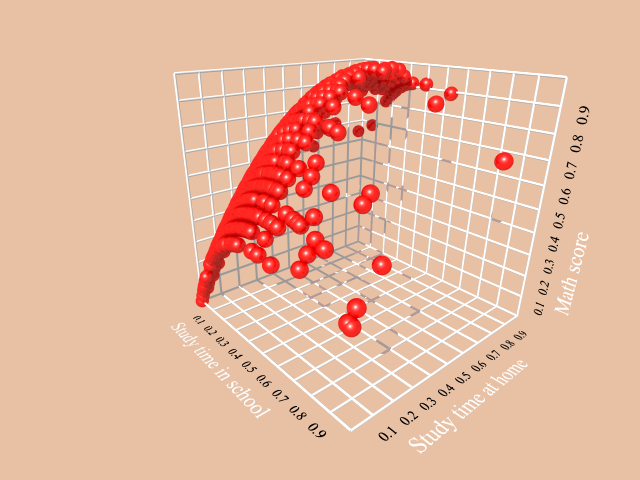
This looks much nicer than a simple plot of the points but still retains the same amount of information. To produce a plot with a perspective that is closer to the one in the last post, the position of the camera has to be changed.

camera{
  location<-0.6, 1.4, -1.0>
  look_at<0.25, 0.5, 0.5>
}

Rendering the scene again yields:

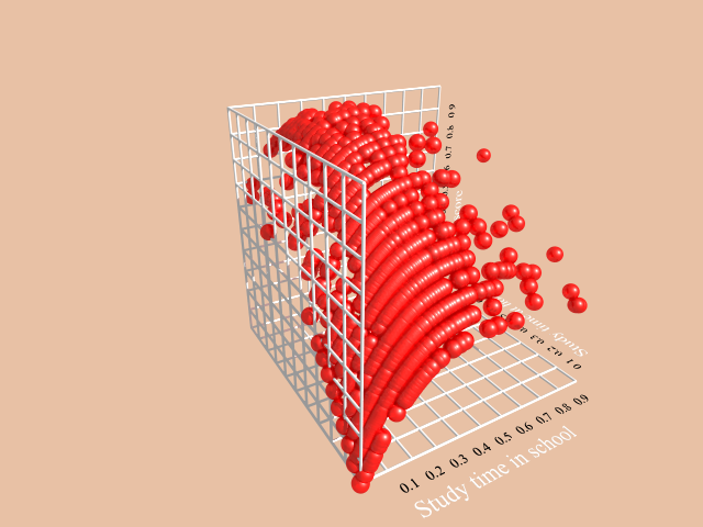
While looking pleasantly, the last two plots still clearly exhibit a scientific "spirit". They have a coordinate system and axis labels with appropriate numbering that makes it possible to extract information about the data that is plotted. To not distract too much from the labels, the overall design is rather plain. With the potential of POVray, however, much more advanced graphics are possible to create something more artistic.

Instead of a full coordinate system for example, we can just use simple axes and add a plane as a basis that causes some reflection of the light rays.

camera{
  location<-1.0, 1.2, -1.8>
  look_at<0.25, 0.25, 0.5>
}

light_source{
  <100, 200, -200> color White
}

background{color LightWood}

plane{
  <0, 1, 0>, -0.01
  pigment{color LightWood}
  finish{reflection 0.3}
}

Disp_Coord_Axes(
  0, 1.0,
  0, 1.0,
  0, 1.0,
  0.005, White
) 

Plot3d(Time_School, Score, Time_Home, Red, 0.03)

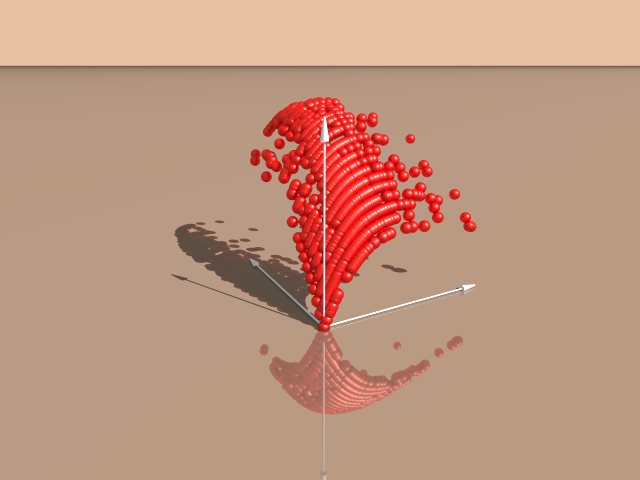
This graphic looks more sophisticated but is not as informative. A graph like this could nevertheless serve to spike some interest in the underlying data.

Animation

In 3D plots like the ones seen above the position of the camera relative to the objects is of crucial importance for the overall look of the image. To get a view from all sides we can either move the camera around the scene or keep the camera in place and rotate the graph.

A nice feature of POVray makes it possible to do exactly that and to create a series of images that can be combined to make an animation. All that has to be done is to build an "animation loop" that outputs a pre-defined number of individual frames. POVray uses a clock counter for this purpose that is controlled by a special text file.

As an example we can modify the code for the scene of the last example to rotate the plot around the y-axis.

// First create a "plot" object
#local plot=union{
  Disp_Coord_Axes(
    0, 1.0, 
    0, 1.0,
    0, 1.0,
    0.005, White
  )

  Plot3d(Time_School, Score, Time_Home, Red, 0.03)
}

// Now rotate the object by increments of the clock counter
object{
  plot
  rotate<0, 360*clock, 0>
}

The associated animation file is called PISAplot.ini but can have any filename ending with .ini. It is a text file that contains the necessary information about the clock variable. In this example I am going to create 30 individual images.

; POV-Ray animation ini file
Antialias=Off

Input_File_Name="PISAplot.pov"

Initial_Frame=1
Final_Frame=30
Initial_Clock=0
Final_Clock=1

Cyclic_Animation=On
Pause_when_Done=Off

Once all the images are rendered they have to be combined to create the movie. If you are using a Unix environment and have ImageMagick installed this can be simply done from the command line.

convert -loop 0 PISAplot*.png PISAplot.gif

The result is a nice gif that can be directly displayed on GitHub pages.

This way the plot can be looked at from all sides to get a feeling for the three-dimensional distribution of the data points.

All these examples are just meant to illustrate the potential of POVray as a "plotting device". The possibilities are endless ranging from a simple plot of data points to nice images of abstract shapes or contours.